Creating a crosstab worksheet in Discoverer Plus:
The following steps will walk you through the process of creating a crosstab worksheet:
- On the first screen of the wizard, select the Crosstab radio button, leaving all the other settings at their default:
Click Next to continue.
- On the Select Items screen of the wizard, you have to select the items you want to include in the workbook, moving them from the Available pane to the Selected:
- So, expand the Orderitems\Quantity node in the Available pane, and right-click the Detail In the pop-up menu, select Add to Worksheet.
- Do the same with the Orderitems\Unitprice
- Expand the Orders node in the Available pane, and right-click the Empid In the pop-up menu, select Add to Worksheet.
- Do the same with the Orders\Orddate
- Expand the Products node in the Available pane, and right-click the Prodname In the pop-up menu, select Add to Worksheet.
- Expand the Salespersons node in the Available pane, and right-click the Name In the pop-up menu, select Add to Worksheet.
- Once you’re done, the Select Items screen of the wizard should look like the following:
Click Next to continue.
- The first thing you should see upon transition to the next screen is the message box informing you that no data can be displayed in the crosstab. Just click OK to close it.
- On the Crosstab Layout screen, you can change the worksheet’s layout. For now, just click Next to continue. Close the message box that should pop up at this point again.
- On the last screen of the wizard, click Finish to complete the creation of the workbook.
Creating a calculation
Here are the steps to follow:
- On the Calculations tab, right-click the My Calculations item, and select New Calculation… in the pop-up menu.
- In the Item Navigator, move to the Calculations tab.
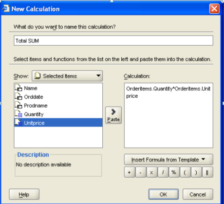
- In the New Calculation dialog, enter the name Total SUM for the calculation. Next, move the Quantity item from the Selected Items pane to the Calculation pane by double-clicking it and then clicking the X button located under the Calculation pane. Finally, double-click the Unitprice item in the Selected Items pane to complete the formula. By now, the New Calculation dialog should look like this
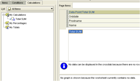
Once you’re done with the formula, click OK to close the New Calculation dialog. As a result, the Total SUM calculation should appear under the My Calculations node on the Calculations tab. Also, the Total SUM column should appear in the worksheet layout.
Changing the worksheet layout:
- First let’s remove the Quantity and Unitprice columns from the worksheet. So, select the Quantity column and hit Delete to remove it from the layout. Do the same with the Unitprice. At this point, the worksheet should look like the following one:
As you can see in the screenshot, there are three items on the top axis and there is no left axis item.
Let’s move an item from the top axis to the left axis. Say, let’s do that with the Prodname item, by dragging it to the left axis, just between the Name and Orddate items.
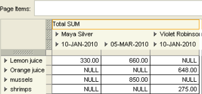
As a result of the previous operation, you should see that a dataset has appeared in the worksheet:
- Right-click any cell on the worksheet and select Format Data… in the pop-up menu.
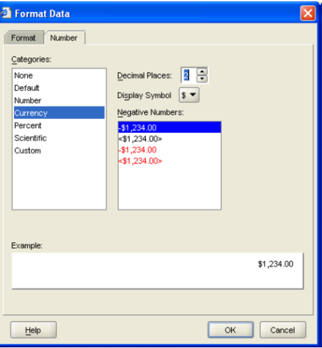
- In the Format Data dialog, move to the Number tab and select the Currency category. Then, increase the Decimal Places to 2 as shown in the following screenshot:
Click OK to change the format and close the dialog. Now if you look at the worksheet, you should see that each number is followed by the $ sign and has two decimal places for cents.
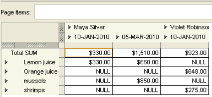
- Move the Total SUM item from the top axis to the left axis. The result should look like this:
As you can see, the worksheet now aggregates the sales figures grouped by product for each date across salespersons.
No comments:
Post a Comment