Performance Tuning for Transformation in Informatica

Joiner Transformation -

• Always prefer to perform joins in the database if possible, as database joins are faster than joins created in Informatica joiner transformation.
• Sort the data before joining if possible, as it decreases the disk I/O performed during joining.
• Make the table with less no of rows as master table.

Lookup Transformation –

• Create an index for the column in a lookup table which is used in lookup condition. Since the lookup table will be queried for looking up the matching data, adding an index would increase the performance.
• If possible, instead of using lookup transformation use join in the database. As database joins are faster, performance will be increased.
• Delete unnecessary columns from the lookup table and keep only the required columns. This will bring down the overhead of fetching the extra columns from the database.

Filter Transformation –

• Use filter transformation as early as possible inside the mapping. If the unwanted data can be discarded early in the mapping, it would increase the throughput.'
• Use source qualifier to filter the data. You can also use source qualifier SQL override to filter the records, instead of using filter transformation.

Aggregator Transformation

• Filter the data before aggregating it. If you are using filter transformation in the mapping, then filter the data before using aggregator as it will reduce the unnecessary aggregation operation.
• Limit the no of ports used in the aggregator transformation. This will reduce the volume of data that aggregator transformation stores inside the cache.

Source Qualifier Transformation

• Bring only the required columns from the source. Most of the times not all the columns of the source table are required, so bring only the required fields by deleting the unnecessary columns.
• Avoid using order by clause inside the source qualifier SQL override. The order by clause requires additional processing and performance can be increased by avoiding it.

Normalizer Transformation in Informatica

Normalizer transformation is a smart way of representing your data in more organized manner. It is used to convert a single row into multiple rows and vice versa. If in a single row there is repeating data in multiple columns, then it can be split into multiple rows. Sometimes we have data in multiple occurring columns. For example

Student Name	Class 9 Score	Class 10 Score	Class 11 Score	Class 12 Score
Student 1	50	60	65	80
Student 2	70	64	83	77

In this case, the class score column is repeating in four columns. Using normalizer, we can split these in the following data set.

Student Name	Class	Score
Student 1	9	50
Student 1	10	60
Student 1	11	65
Student 1	12	80
Student 2	9	70
Student 2	10	64
Student 2	11	83
Student 2	12	77

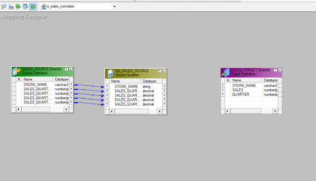
Step 1 – Create source table "sales_source" and target table "sales_target" using the script and import them in Informatica

drop table sales_source;drop table sales_target;CREATE TABLE sales_source (  store_name varchar2(20),   sales_quarter1 NUMBER(5),  sales_quarter2 NUMBER(5),  sales_quarter3 NUMBER(5),  sales_quarter4 NUMBER(5));  create table sales_target ( store_name varchar2(20), sales number(5), quarter number(3) );insert into sales_source values ( 'DELHI',150, 240, 450, 100);insert into sales_source values ( 'MUMBAI',100, 500, 350, 340);COMMIT;/

Step 2 – Create a mapping having source "sales_source" and target table "sales_target"

Step 3 – From the transformation menu create a new transformation

1. Select normalizer as transformation
2. Enter name, "nrm_sales"
3. Select create option

Step 4 – The transformation will be created, select done option

Step 5 – Double click on the normalizer transformation, then

1. Select normalizer tab
2. Click on icon to create two columns
3. Enter column names
4. Set number of occurrence to 4 for sales and 0 for store name
5. Select OK button

Columns will be generated in the transformation. You will see 4 number of sales column as we set the number of occurrences to 4.

Step 6 – Then in the mapping

1. Link the four column of source qualifier of the four quarter to the normalizer columns respectively.
2. Link store name column to the normalizer column
3. Link store_name & sales columns from normalizer to target table
4. Link GK_sales column from normalizer to target table

Save the mapping and execute it after creating session and workflow. For each quarter sales of a store, a separate row will be created by the normalizer transformation.

The output of our mapping will be like –

Store Name	Quarter	Sales
DELHI	1	150
DELHI	2	240
DELHI	3	455
DELHI	4	100
MUMBAI	1	100
MUMBAI	2	500
MUMBAI	3	350
MUMBAI	4	340

The source data had repeating columns namely QUARTER1, QUARTER2, QUARTER3, and QUARTER4. With the help of normalizer, we have rearranged the data to fit into a single column of QUARTER and for one source record four records are created in the target.

In this way, you can normalize data and create multiple records for a single source of data.

Lookup and Re-usable transformation in Informatica

Lookup transformation provides the feature to lookup matching values in a table based on the values in source data. Basically, it's a kind of join operation in which one of the joining table is the source data, and the other joining table is the lookup table.

In previous topics, we used joiner transformation to join "emp" and "dept" table to bring department names.

In this section, we will implement the same using lookup transformation.

Step 1 – Create a new mapping with EMP as source and EMP_DEPTNAME as target

Step 2 – Create a new transformation using transformation menu then

1. Select lookup transformation as the transformation
2. Enter transformation name "lkp_dept"
3. Select create option

Step 3 – This will open lookup table window, in this window

1. Select source button
2. Select DEPT table
3. Select Ok Button

Step 4 - Lookup transformation will be created with the columns of DEPT table, now select done button

Step 5 - Drag and drop DEPTNO column from source qualifier to the lookup transformation, this will create a new column DEPTNO1 in lookup transformation. Then link the DNAME column from lookup transformation to the target table.

The lookup transformation will lookup and return department name based upon the DEPTNO1 value.

Step 6 – Double click on the lookup transformation. Then in the edit transformation window

1. Select condition tab
2. Set the condition column to DEPTNO = DEPTNO1
3. Select Ok Button

Step 7 – Link rest of the columns from source qualifier to the target table

Now, save the mapping and execute it after creating the session and workflow. This mapping will fetch the department names using lookup transformation.

The lookup transformation is set to lookup on dept table. And the joining condition is set based on dept number.

Reusable Transformation

A normal transformation is an object that belongs to a mapping and can be used inside that mapping only. However, by making a transformation reusable it can be re-used inside several mappings.

For example, a lookup transformation which fetches employee details based on employee number can be used at multiple mappings wherever employee details are required.

By using reusable transformation, it reduces the overwork of creating same functionality again.

To make a transformation reusable –

Step 1 – Open the mapping which is having the transformation, here we are making the rank transformation reusable.

Step 2 – Double click on the transformation to open edit transformation window. Then

1. Select Transformation tab in the window
2. Select the check box to make transformation reusable
3. Select yes in the confirmation window
4. Select OK in the transformation properties window.

This will make the transformation reusable.

Transaction Control Transformation in Informatica

Transaction control transformation allows us to commit or rollback transactions during the execution of the mapping.

Commit and rollback operations are of significant importance as it guarantees the availability of data.

When processing a high volume of data, there can be a situation when to commit the data to the target.

If a commit is performed too frequently, then it will be an overhead to the system. If a commit is performed too late then in case of failure there are chances of data loss.

So to provide flexibility Transaction control transformation is provided. There are five in built variables available in this transformation to handle the operation.

1. TC_CONTINUE_TRANSACTION
   In tc_continue_transaction there are no operations performed, the process of data load continues as it is
2. TC_COMMIT_BEFORE
   In tc_commit_before when this flag is found set, a commit is performed before the processing of current row.
3. TC_COMMIT_AFTER
   In tc_commit_after the current row is processed then a commit is performed.
4. TC_ROLLBACK_BEFORE
   In tc_rollback_before, rollback is performed first then data is processed to write
5. TC_ROLLBACK_AFTER
   In tc_rollback_after data is processed then the rollback is performed.

In this example, we will commit data to the target when dept no =20 condition is found true

Step 1 – Create a mapping with EMP as source and EMP_TARGET as target

Step 2 – Create a new transformation using transformation menu, then

1. Select a transaction control as the new transformation
2. Enter transformation name "tc_commit_dept20"
3. Select create option

Step 3 – The transaction control transformation will be created, select done button

Step 4 - Drag and drop all the columns from source qualifier to the transaction control transformation then link all the columns from transaction control transformation to the target table

Step 5 – Double click on the transaction control transformation and then in the edit property window

1. Select property tab
2. Click on the transaction control editor icon

Step 6 –in the expression editor enter the expression –

"iif(deptno=20,tc_commit_before,tc_continue_transaction)" and select OK

It means if deptno 20 is found then commit transaction in target, else continue the current processing.

Step 7 – Select OK in the previous window

Now save the mapping and execute it after creating session and workflows. This mapping will commit the data to the target whenever department number 20 is found in the data.

Sequence Generator Transformation in Informatica

Sequence generator transformation is used to generate numeric sequence values like 1, 2, 3, 4, 5 etc.

For example, you want to assign sequence values to the source records, then you can use sequence generator. The generated sequence values can be like 5, 10, 15, 20, 25 etc. or 10, 20, 30, 40, 50 etc. depending upon the configured properties of the transformation.

The sequence generator is also used to generate primary key values. It is a passive transformation & it does not affect the number of input rows.

It has two output ports

• CURRVAL
• NEXTVAL

CURRVAL port value is always NEXTVAL+1.

To generate the sequence numbers, we always use the NEXTVAL column.

Properties of Sequence Generator Transformation

• Start Value – It is the first value that will be generated by the transformation, the default value is 0.
• Increment by – This is the number by which you want to increment the values. The default value is 1.
• End value – It is the maximum value that the transformation should generate.
• Cycle – if this option is set then after reaching the end of the value, the transformation restarts from the start value.

In this example, we will generate sequence numbers and store in the target.

Step 1 – Create a target table with the following script.

DROP TABLE EMP_SEQUENCE;

CREATE TABLE EMP_SEQUENCE(

 EMPNO NUMBER(4) NOT NULL,

 ENAME VARCHAR2(10),

 JOB VARCHAR2(9),

 MGR NUMBER(4),

 HIREDATE DATE,

 SAL NUMBER(7, 2),

 COMM NUMBER(7, 2),

 DEPTNO NUMBER(2),

 SNO NUMBER(3)

) ;

PURGE RECYCLEBIN

/

Step 2- Import the table in Informatica as target table

Step 3 – Create a new mapping and import EMP source and EMP_SEQUENCE target table

Step 4 – Create a new transformation in the mapping

1. Select sequence transformation as the type
2. Enter transformation name "seq_emp"
3. Select Create option

Step 5 - Sequence generator transformation will be created, select the done option

Step 6 - Link the NEXTVAL column of sequence generator to SNO column in target

Step 7 – link the other columns from source qualifier transformation to the target table

Step 8 – Double click on the sequence generator to open property window, and then

1. Select the properties tab
2. Enter the properties with Start value =1, leave the rest properties as default
3. Select OK button

Now save the mapping and execute it after creating the session and workflow.

The sno column in the target would contain the sequence numbers generated by the sequence generator transformation.

In our example, the sequences will be like 1 – Scott, 2 – King, 3 – Adam, 4 – Miller, etc.

Tableau: A leading data visualization tool

Tableau is a Business Intelligence tool for visually analyzing the data. Users can create and distribute interactive and shareable dashboards which depict the trends, variations and density of the data in form of graphs and charts. Tableau can connect to files, relational and Big data sources to acquire and process data. The software allows data blending and real time collaboration, which makes it very unique. It is used by businesses, academic researchers and many governments to do visual data analysis. It is also positioned as a leader Business Intelligence and Analytics Platform in Gartner Magic Quadrant.

As a leading data visualization tool Tableau has many desirable and unique features. Its powerful data discovery and exploration application allows you to answer important questions in seconds. You can use Tableau's drag and drop interface to visualize any data, explore different views, and even combine multiple databases together easily. It does not need any complex scripting. Anyone who understands the business problem can address it with a visualization of the relevant data. When the analysis is finished, sharing with others is as easy as publishing to Tableau Server.

Tableau Features

Tableau provides solutions for all kinds of industries, departments and data environments. Below are the unique features which enable tableau handle so many diverse scenarios.

• Speed of Analysis - As it does not need high level of programming expertise, any computer user with access to data can start using it to derive value from the data.
• Self-Reliant - Tableau does not need a complex software setup. The desktop version which is used by most users is easily installed and contains all the features needed to start and complete data analysis.
• Visual Discovery - The user explores and analyses the data by using visual tools like colours, trend lines, charts and graphs. There is very little script to be written as nearly everything is done by drag and drop.
• Blend Diverse Data Sets - Tableau allows you to blend different relational, semi-structured and raw data sources in real time, without expensive up-front integration costs. The users don’t need to know the details of how data is stored.
• Architecture Agnostic - Tableau works in all kinds of devices where data flows. So the user need not worry about specific hardware or software requirements to use Tableau.
• Real Time Collaboration - Tableau can filter, sort, and discuss data on the fly and embed a live dashboard in portals like SharePoint site or Salesforce. You can save your view of data and allow colleagues to subscribe to your interactive dashboards so they see the very latest data just by refreshing their web browser.
• Centralized Data - The tableau server provides a centralized location to manage all of the organization’s published data sources. You can delete, change permissions, add tags, and manage schedules in one convenient location. It’s easy to schedule extract refreshes and manage them in the data server. Administrators can centrally define a schedule for extracts on the server for both incremental and full refreshes.

For More information, please go through the below link:

My Tableau Presentation

Rank Transformation in Informatica

Rank Transformation performs the filtering of data based on group and ranks.

For example, you want to get ten records of employees having highest salary, such kind of filtering can be done by rank transformation.

Rank transformation also provides the feature to do ranking based on groups. Like if you want to get top ten salaried employee department wise, then this grouping can be done with this transformation.

Rank transformation is an active transformation, as it affects the number of output rows.

The rank transformation has an output port by which it assigns a rank to the rows.

Our requirement is to load top 3 salaried employees for each department; we will implement this using rank transformation.

Step 1 - Create a mapping having source EMP and target EMP_TARGET

Step 2- Then in the mapping

1. Select transformation menu
2. Select create option

Step 3 – In the create transformation window

1. Select rank transformation
2. Enter transformation name "rnk_salary"
3. Select Create button

Step 4 – The rank transformation will be created in the mapping, select done button in the window

Step 5 – Connect all the ports from source qualifier to the rank transformation

Step 6- Double click on the rank transformation and it will open "edit transformation window". In this window

1. Select properties menu
2. Select "Top" option from the Top/Bottom property
3. Enter 3 in the number of ranks

Step 7 – In the "edit transformation" window again

1. Select ports tab
2. Select group by option for the deptno column
3. Select ok button

Step 8 –Connect the ports from rank transformation to the target table

Now, save the mapping and execute it after creating session and workflow. The source qualifier will fetch all the records, but rank transformation will pass only records having three high salaries for each department.

Joiner transformation in Informatica

The joiner transformation provides you the option to create joins in Informatica. The joins created using joiner transformation are similar to the joins in databases. The advantage of joiner transformation is that joins can be created for heterogeneous systems (different databases).

In joiner transformation, there are two sources which we are going to use it for joins. These two sources are called

• Master Source
• Detail Source

In the properties of joiner transformation, you can select which data source can be Master and which source can be detail source.

During execution, the master source is cached into the memory for joining purpose. So it is recommended to select the source with less number of records as the master source.

The following joins can be created using joiner transformation

1. Master outer join
   In Master outer join, all records from the Detail source are returned by the join and only matching rows from the master source are returned.
2. Detail outer join
   In detail outer join only matching rows are returned from the detail source, and all rows from the master source are returned.
3. Full outer join
   In full outer join, all records from both the sources are returned. Master outer and Detail outer joins are equivalent to left outer joins in SQL.
4. Normal join
   In normal join only matching rows are returned from both the sources.

In this example, we will join emp and dept tables using joiner transformation

Step 1 – Create a new target table EMP_DEPTNAME in the database using the below script and import the table in Informatica targets.

DROP TABLE EMP_DEPTNAME;

CREATE TABLE EMP_DEPTNAME(

 EMPNO NUMBER(4) NOT NULL,

 ENAME VARCHAR2(10),

 JOB VARCHAR2(9),

 MGR NUMBER(4),

 HIREDATE DATE,

 SAL NUMBER(7, 2),

 COMM NUMBER(7, 2),

 DEPTNO NUMBER(2),

 DEPTNAME VARCHAR2(30)

) ;

PURGE RECYCLEBIN

/

Step 2 - Create a new mapping and import source tables "EMP" and "DEPT" and target table which we created in the previous step

Step 3 – From the transformation menu, select create option.

1. Select joiner transformation
2. Enter transformation name "jnr_emp_dept"
3. Select create option

Step 4 – Drag and drop all the columns from both the source qualifiers to the joiner transformation

Step 5 - Double click on the joiner transformation, then in the edit transformation window

1. Select condition tab
2. Click on add new condition icon
3. Select deptno in master and detail columns list

Step 6 - Then in the same window

1. Select properties tab
2. Select normal Join as join type
3. Select OK Button

For performance optimization, we assign the master source to the source table pipeline which is having less no of records. To perform this task –

Step 7 –Double click on the joiner transformation to open edit properties window, and then

1. Select ports tab
2. Select any column of a particular source which you want to make a master
3. Select OK 

Step 8 – Link the relevant columns from joiner transformation to target table

Now save the mapping and execute it after creating session and workflow for it. The join will be created using Informatica joiner, and relevant details will be fetched from both the tables.