OBIEE: Working with Database Data

Using analytic SQL functions:

Analytic SQL is one of those Oracle Database native features that you can start using immediately after installing the database.

For example, you might need to know how many employees in your organization have been working for the company for 15 years or more. In this example, you might query the employees table located in the hr/hr demonstration schema, issuing the following statement:

SELECT count(*) FROM employees WHERE (EXTRACT(YEAR FROM (SYSDATE)) -

EXTRACT(YEAR FROM (hire_date))) >= 15;

The output should look like this:

COUNT(*)

———-

17

Multidimensional data analysis with SQL:

To start with, let’s create a new database schema, and the tables within it that are needed for this example. You can perform all these tasks from SQL*Plus. First, you have to launch SQLPLUS. This can be done from within an operating system prompt as follows:

C:\oracle\...>sqlplus

When prompted, you have to connect as sysdba:

Enter user-name: /as sysdba

Once connected as sysdba, you can issue the following statements to create a new schema and grant it the privileges required for this example:

CREATE USER usr IDENTIFIED BY usr;

GRANT connect, resource TO usr;

CONN usr/usr

Before you can proceed to the example, you need to define some tables in the newly created database schema. For example, you might create the following tables: salespersons, regions, and orders related to one another through the foreign keys defined in the orders table. Here is the SQL code to issue:

CREATE TABLE salespersons (

emp_id VARCHAR2(10) PRIMARY KEY,

emp_name VARCHAR2(40)

);

CREATE TABLE regions (

reg_id VARCHAR2(2) PRIMARY KEY,

reg_name VARCHAR2(20)

);

CREATE TABLE orders(

ordno NUMBER PRIMARY KEY,

empid VARCHAR2(10) REFERENCES salespersons(emp_id),

regid VARCHAR2(2) REFERENCES regions(reg_id),

orddate DATE,

total NUMBER(10,2)

);

Next, you have to populate these tables with some data, so that you can perform queries against them. As the orders table refers to the salespersons and regions tables, you first have to populate these two tables with data. You might use the following statements for this:

INSERT INTO salespersons VALUES ('violet', 'Violet Robinson');

INSERT INTO salespersons VALUES ('maya', 'Maya Silver');

INSERT INTO regions VALUES ('NA', 'North America');

INSERT INTO regions VALUES ('EU', 'Europe');

The Intellipaat OBIEE developer training is what you need to grab the best jobs in Business Intelligence!

Now that you have filled up the salespersons and regions tables, you can move on and populate the orders table:

INSERT INTO orders VALUES

(1001, 'violet', 'NA', '10-JAN-2010', 1450.00);

INSERT INTO orders VALUES

(1002, 'violet', 'NA', '15-JAN-2010', 2310.00);

INSERT INTO orders VALUES

(1003, 'maya', 'EU', '20-JAN-2010', 1480.00);

INSERT INTO orders VALUES

(1004, 'violet', 'NA', '19-FEB-2010', 3700.00);

INSERT INTO orders VALUES

(1005, 'maya', 'EU', '24-FEB-2010', 1850.00);

INSERT INTO orders VALUES

(1006, 'maya', 'EU', '04-MAR-2010', 1770.00);

INSERT INTO orders VALUES

(1007, 'maya', 'EU', '05-MAR-2010', 1210.50);

INSERT INTO orders VALUES

(1008, 'violet', 'NA', '05-MAR-2010', 10420.00);

COMMIT;

You now have all the parts required to proceed with the example, and can issue a query that summarizes sales figures for every region for each month. Here is what this query might look like:

SELECT r.reg_name region, TO_CHAR(TO_DATE(EXTRACT(MONTH FROM (o.orddate)),'MM'),'Month') month, SUM(o.total) sales

FROM regions r, orders o

WHERE r.reg_id = o.regid

GROUP BY ROLLUP(EXTRACT(MONTH FROM (o.orddate)), r.reg_name);

The query results should look like this:

REGION	MONTH	SALES
Europe	January	1480
North America	January	3760
January		5240
Europe	February	1850
North America	February	3700
	February	5550
Europe	March	2980.5
North America	March	10420
	March	13400.5
		24190.5
	March	10420

Changing the order in which the parameters of ROLLUP appear will also affect the report. In our example, if you move the r.reg_name parameter to the first position, the report will generate totals for each region rather than for each month. Here is the query:

SELECT r.reg_name region, TO_CHAR(TO_DATE(EXTRACT(MONTH FROM (o.orddate)),'MM'),'Month') month, SUM(o.total) sales

FROM regions r, orders o

WHERE r.reg_id = o.regid

GROUP BY ROLLUP(r.reg_name, EXTRACT(MONTH FROM (o.orddate)));

Here is its output:

REGION	MONTH	SALES
Europe	January	1480
Europe	February	1850
Europe	March	2980.5
Europe		6310.5
North America	January	3760
North America	February	3700
North America	March	10420
North America		17880
		24190.5

As you can see, in the above report there are no longer any month totals. Instead, it provides you with the totals for each region.

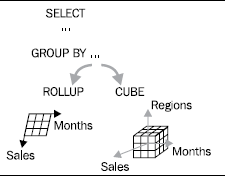
Cubing:

The following figure gives a graphical depiction of how CUBE differs from ROLLUP when it comes to generating summary information:

Switching to SQL, you might write the following query using the CUBE function in the GROUP BY clause:

SELECT r.reg_name region, TO_CHAR(TO_DATE(EXTRACT(MONTH FROM (o.orddate)),'MM'),'Month') month, SUM(o.total) sales

FROM regions r, orders o

WHERE r.reg_id = o.regid

GROUP BY CUBE(EXTRACT(MONTH FROM (o.orddate)), r.reg_name);

The previous query should generate the following report:

REGION	MONTH	Sales
Europe	January	1480
North America	January	3760
	January	5240
Europe	February	1850
North America	February	3700
	February	5550
Europe	March	2980.5
North America	March	10420
	March	13400.5
Europe		6310.5
North America		17880
		24190.5

As you can see, you now have all possible subtotals and totals combinations presented in the report. This is why changing the order of columns in CUBE won’t affect the report, unlike with ROLLUP. So, the following query should actually give you the same results as above:

SELECT r.reg_name region, TO_CHAR(TO_DATE(EXTRACT(MONTH FROM (o.orddate)),'MM'),'Month') month, SUM(o.total) sales

FROM regions r, orders o

WHERE r.reg_id = o.regid

GROUP BY CUBE(r.reg_name, EXTRACT(MONTH FROM (o.orddate)));

However, the order of rows in the report will be a little different:

REGION	MONTH	SALES
Europe	January	1480
Europe	February	1850
Europe	March	2980.5
Europe		6310.5
North America	January	3760
North America	February	3700
North America	March	10420
North America		17880
January		5240
February		5550
March		13400.5
		24190.5

Generating reports with only summary rows:

In some cases, you may not need to include the rows that represent the subtotals generated by GROUP BY, but include only the total rows. This is where the GROUPING SETS extension of the GROUP BY clause may come in handy:

SELECT r.reg_name region, TO_CHAR(TO_DATE(EXTRACT(MONTH FROM (o.orddate)),'MM'),'Month') month, SUM(o.total) sales

FROM regions r, orders o

WHERE r.reg_id = o.regid

GROUP BY GROUPING SETS(r.reg_name, EXTRACT(MONTH FROM (o.orddate)));

This query should produce the following report:

REGION	MONTH	SALES
North America		17880
Europe		6310.5
	January	5240
	February	5550
	March	13400.5

Ranking:

To better understand how ranking works, though, let’s first look at the query that simply summarizes sales figures per region:

SELECT r.reg_name region, SUM(o.total) sales

FROM regions r, orders o

WHERE r.reg_id = o.regid

GROUP BY GROUPING SETS(r.reg_name);

Here is the output you should see:

Region	Sales
North America	17880
Europe	6310.5

Now let’s look at the query that will compute a sales rank for each region in ascending order:

SELECT r.reg_name region, SUM(o.total) sales, RANK() OVER (ORDER BY

SUM(o.total) ASC) rank

FROM regions r, orders o

WHERE r.reg_id = o.regid

GROUP BY GROUPING SETS(r.reg_name);

 This time, the query results should look like this:

Region	Sales	Rank
Europe	6310.5	1
North America	17880	2

 Windowing:

Windowing functions make up another important group of analytic SQL functions. The idea behind windowing functions is that they enable aggregate calculations to be made within a “sliding window” that may float down as you proceed through the result set.

SELECT TO_CHAR(TO_DATE(EXTRACT(MONTH FROM (o.orddate)),'MM'),'Month')

month, SUM(o.total) sales,

AVG(SUM(o.total)) OVER (ORDER BY TO_CHAR(TO_DATE(EXTRACT(MONTH FROM

(o.orddate)),'MM'),'Month') ROWS BETWEEN 1 PRECEDING AND 1 FOLLOWING)

sliding_avg

FROM orders o

GROUP BY TO_CHAR(TO_DATE(EXTRACT(MONTH FROM (o.orddate)),'MM'),'Month

');

 The output should look like the following:

MONTH	SALES	SLIDING_AVG
February	5550	5395
January	5240	8063.5
March	13400.5	9320.25

 Aside from the AVG function, you can apply the windowing technique using the other aggregate functions, such as SUM, MIN, and MAX.

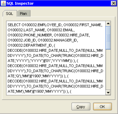
 Discovering SQL in Discoverer:

Discoverer use SQL behind the scenes. Although you won’t see any SQL code immediately after a visual IDE has been loaded, it’s no more than 1 or 2 clicks away. In Discoverer Plus, for example, you can look at the SQL code behind a Discoverer item through the SQL Inspector, which you can launch by clicking the Tools\Show SQL menu. As an example, the SQL Inspector dialog containing the SQL behind the hr.employees item is shown in the following figure: